Explorez le calcul numérique en Swift avec MLX

3:04 - Power iteration with MLX Swift arrays

import MLX
let n = 100
let steps = 10
let B = MLXRandom.normal([n, n])
var v = MLXRandom.normal([n])

// get symmetric matrix A = Bᵀ + B
let A = B.T + B

// Power iteration → top eigenvector of A.
//   v ← A v / ‖A v‖
for _ in 0 ..< steps {
    let Av = matmul(A, v)
    v = Av / norm(Av)
    eval(v)
}

// recover the eigenvalue.
//   λ = vᵀ A v
let lambda = matmul(matmul(v.T, A), v)

print(lambda)

5:09 - Mandelbrot set in plain Swift (scalar)

// Plain Swift, scalar-at-a-time
var counts = Array2D<Int>(width: w, height: h)

for y in 0 ..< h {
    for x in 0 ..< w {
        let c = Complex(xMin + Float(x) * xStep, yMin + Float(y) * yStep)
        var z = Complex<Float>.zero
        var limit = maxIterations
        for i in 0 ..< maxIterations {
            z = z * z + c
            if z.lengthSquared > radiusSquared {
                limit = i
                break
            }
        }
        counts[x, y] = limit
    }
}

5:27 - Mandelbrot set in MLX Swift (array)

// Compute the Mandelbrot set on a grid of complex numbers
import MLX

let x = linspace(-2.0, 0.5, count: w)
let y = linspace(-1.25, 1.25, count: h).reshaped(h, 1)
let c = x + y.asImaginary()

var z = MLXArray.zeros(like: c)
var counts = MLXArray.zeros(c.shape, dtype: .int16)

for _ in 0 ..< maxIterations {
    z = z * z + c                       // iterate z ← z² + c
    counts = counts + (abs(z) .< 2)     // count bounded iterations
}

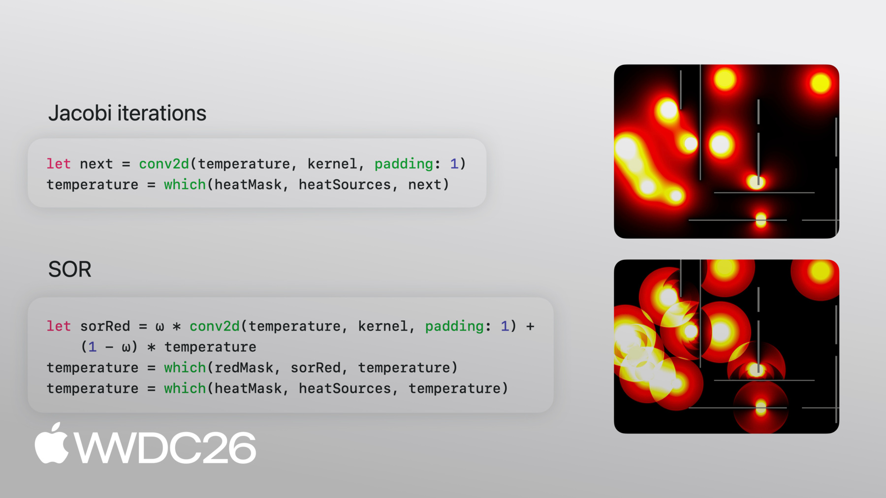
7:27 - Jacobi iteration with conv2d

// Jacobi iteration: average the four neighbors

// Convolution weights
let kernel = MLXArray(converting: [
    0,    0.25, 0,
    0.25, 0,    0.25,
    0,    0.25, 0,
]).reshaped(1, 3, 3, 1)

// Initial value
var temperature = heatSources

// Run this in a loop until convergence
let next = conv2d(temperature, kernel, padding: 1)
temperature = which(heatMask, heatSources, next)

9:17 - Successive Over-Relaxation (SOR)

// Successive Over-Relaxation: blend the previous and next state
let ω: Float = 2.0 / (1.0 + sin(Float.pi / Float(max(M, N))))

let redMask   = checkerboard(rows: M, cols: N, phase: 0)
let blackMask = checkerboard(rows: M, cols: N, phase: 1)

// Update red cells using black neighbors
let sorRed  = ω * conv2d(temperature, kernel, padding: 1) + (1 - ω) * temperature
temperature = which(redMask, sorRed, temperature)
temperature = which(heatMask, heatSources, temperature)

// Update black cells using (now-updated) red neighbors
let sorBlack = ω * conv2d(temperature, kernel, padding: 1) + (1 - ω) * temperature
temperature  = which(blackMask, sorBlack, temperature)
temperature  = which(heatMask, heatSources, temperature)

11:13 - Curve fitting with automatic differentiation

// Define a loss, then optimize it with autodiff
// x, y: data points as MLXArrays
func f(_ θ: MLXArray) -> MLXArray {
    θ[0] + θ[1] * x + θ[2] * x ** 2
}

func loss(_ θ: MLXArray) -> MLXArray {
    mean((f(θ) - y) ** 2)
}

var θ = zeros([numParams])
let gradLoss = grad(loss)

for _ in 0 ..< steps {
    let g = gradLoss(θ)         // ∇L(θ)
    θ = θ - learningRate * g    // parameter update
    eval(θ)                     // force evaluation
}